KKCalc2#
KKCalc2 (xraysoftmat/kkcalc) is another xraysoftmat package for calculating the complex index of refraction of materials using the Kramers-Kronig relations. This makes the calculation of the refractive index for various structures very easy. This package is designed to be used in conjunction with the XEFI package to calculate the X-ray Electric Field Intensity (XEFI) within multi-layer structures.
Usage#
Note that this package is an optional dependency for XEFI and is not required for basic calculations. You can install it using pip:
pip install kkcalc2
or install it alongside the XEFI package:
pip install XEFI --group kk
Atomic Scattering Polynomials (ASP)#
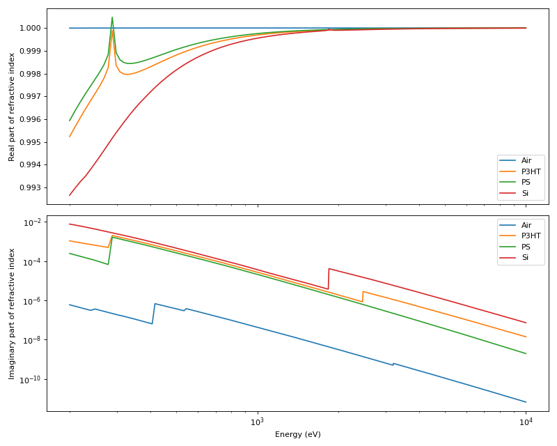
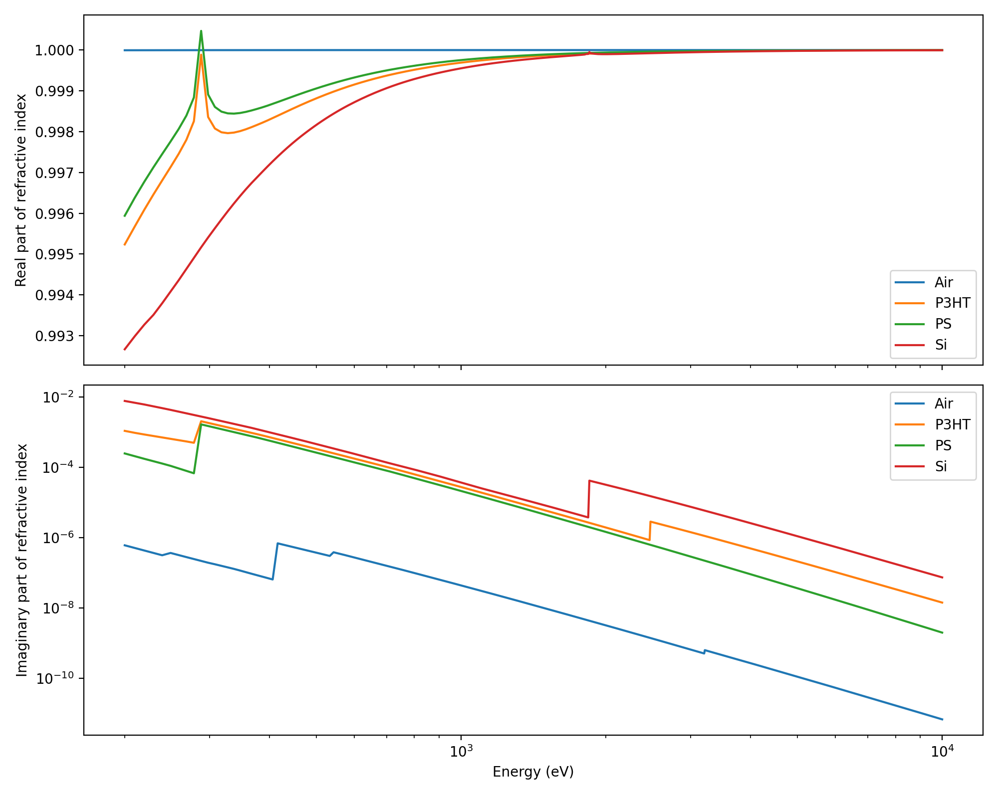
KKCalc2 uses databases (DB) to construct a material’s atomic scattering (AS) factors, which can then be used to calculate the complex index of refraction. See the KKCalc2 documentation for more information on how to use the package and its features.
import matplotlib.pyplot as plt
import numpy as np
from kkcalc2.models import asp_db_complex

# Construct atomic scattering polynomial (ASP) models from database atomic scattering factors for a few materials
refractive_air = asp_db_complex("(N78O20Ar1)0.01", density=0.001225, name="Air")
refractive_P3HT = asp_db_complex("C10H14S", density=1.33, name="P3HT")
refractive_PS = asp_db_complex("C8H8", density=1.05, name="PS")
refractive_Si = asp_db_complex("Si", density=2.329, name="Si")

# Evaluate the real and imaginary parts of the refractive index for a range of energies
energies = np.linspace(200, 10000, 1000)  # Energy range from 200 eV to 10 keV
n_air = refractive_air.eval_refractive_index(energies)
n_P3HT = refractive_P3HT.eval_refractive_index(energies)
n_PS = refractive_PS.eval_refractive_index(energies)
n_Si = refractive_Si.eval_refractive_index(energies)

fig,ax = plt.subplots(2,1, figsize=(10,8), sharex=True)
ax[0].plot(energies, n_air.real, label="Air")
ax[0].plot(energies, n_P3HT.real, label="P3HT")
ax[0].plot(energies, n_PS.real, label="PS")
ax[0].plot(energies, n_Si.real, label="Si")
ax[0].set_ylabel("Real part of refractive index")
ax[0].legend()
ax[1].plot(energies, n_air.imag, label="Air")
ax[1].plot(energies, n_P3HT.imag, label="P3HT")
ax[1].plot(energies, n_PS.imag, label="PS")
ax[1].plot(energies, n_Si.imag, label="Si")
ax[1].set_xlabel("Energy (eV)")
ax[1].set_ylabel("Imaginary part of refractive index")
ax[1].legend()
ax[1].set_yscale("log")
ax[1].set_xscale("log")
ax[0].patch.set_alpha(0)
ax[1].patch.set_alpha(0)
ax[0].patch.set_facecolor('none')
ax[1].patch.set_facecolor('none')
fig.tight_layout()
plt.show()
(Source code, png, hires.png, pdf)

KKCalc2 - XEFI Integration#
The ASP descriptions can then be used to calculate all refractive indexes in a multi-layer model.
# Wavelength / Beam Energy
wav = 1.54  # Å
beam_energy = XEFI.utils.wav2en(wav) # in eV

angles = np.linspace(0.1, 0.4, 3000)  # Angles of Incidence in degrees
z = [0, -800, -1340]  # Z-coordinates for the multilayer interface

# Refractive indexes
refractive_indicies: list[kk.models.asp_complex] = [
    refractive_air,
    refractive_PS,
    refractive_P3HT,
    refractive_Si,
]

result = XEFI.XEF_Basic(
    energies=beam_energy,
    angles=angles,
    z=z,
    refractive_indices=refractive_indicies,
    method=XEFI.XEF_method.DEV,
)

fig, ax = result.generate_graphic_XEFI_map(z_vals)
ax.set_title(
    rf"X-ray Electric Field Intensity at $\lambda$={wav} Å, {beam_energy:0.2f} eV",
    pad=20,
)
plt.show()