Basic#
This tutorial will show how to use the XEF_Basic model to calculate the electric field intensity of a simple multi-layer structure. The XEF_Basic model is a simple model that calculates the electric field intensity of a multi-layer structure using the Fresnel equations and the recursive . It is a good starting point for understanding how to use the XEFI package.
We have two result implementations; BasicResult and BasicRoughResult, which are used for smooth and rough interfaces respectively.
Our structure will consist of Air/Vacuum, Polystyrene (C8H8), Poly(3-hexylthiophene) (P3HT, C10H14S), and a Silicon (Si) substrate. The Si and Air/Vacuum layers are semi-infinite, while the PS and P3HT layers have thicknesses of 800 Å and 540 Å respectively. The z-coordinates of the interfaces are at 0, -800, and -1340 Å respectively.
Let’s define some initial parameters.
import XEFI
import numpy as np

energy = 8050.92 # eV, corresponding to a wavelength of 1.54 Å
angles = np.linspace(0.1, 0.4, 3000) # Angles of Incidence in degrees
z = [0, -800, -1340]  # Z-coordinates for the multilayer interface
layer_names = ["Air", "PS", "P3HT", "Si"]
We can now define the refractive indices for each layer. See KKCalc2 for how to calculate these using the kkcalc2 package.
# Calculated at 8050.92 eV using kkcalc2, but could be any complex
# refractive index or callable that returns a complex refractive index.
refractive_indices = [
    1.0        + 0j,         # Air/Vacuum
    0.99999637 + 4.96e-09j,  # Polystyrene (C8H8)
    0.99999536 + 3.31e-08j,  # Poly(3-hexylthiophene) (P3HT, C10H14S)
    0.99999243 + 1.72e-07j,  # Silicon (Si)
 ]
This sufficiently describes the multi-layer structure, and we can now calculate the electric field intensity using the XEF_Basic method to create a BasicResult class.
BasicResult#
We can now compute the electric field intensity using the XEF_Basic method to create a BasicResult class.
result: XEFI.BasicResult = XEFI.XEF_Basic(
    energies=energy,
    angles=angles,
    z=z,
    refractive_indices=refractive_indices,
    layer_names=layer_names,
)
This object has calculated properties for the model, which are demonstrated in the folloiwng sections. For a full list, refer to the API reference for the BasicResult class.
XEFI Maps#
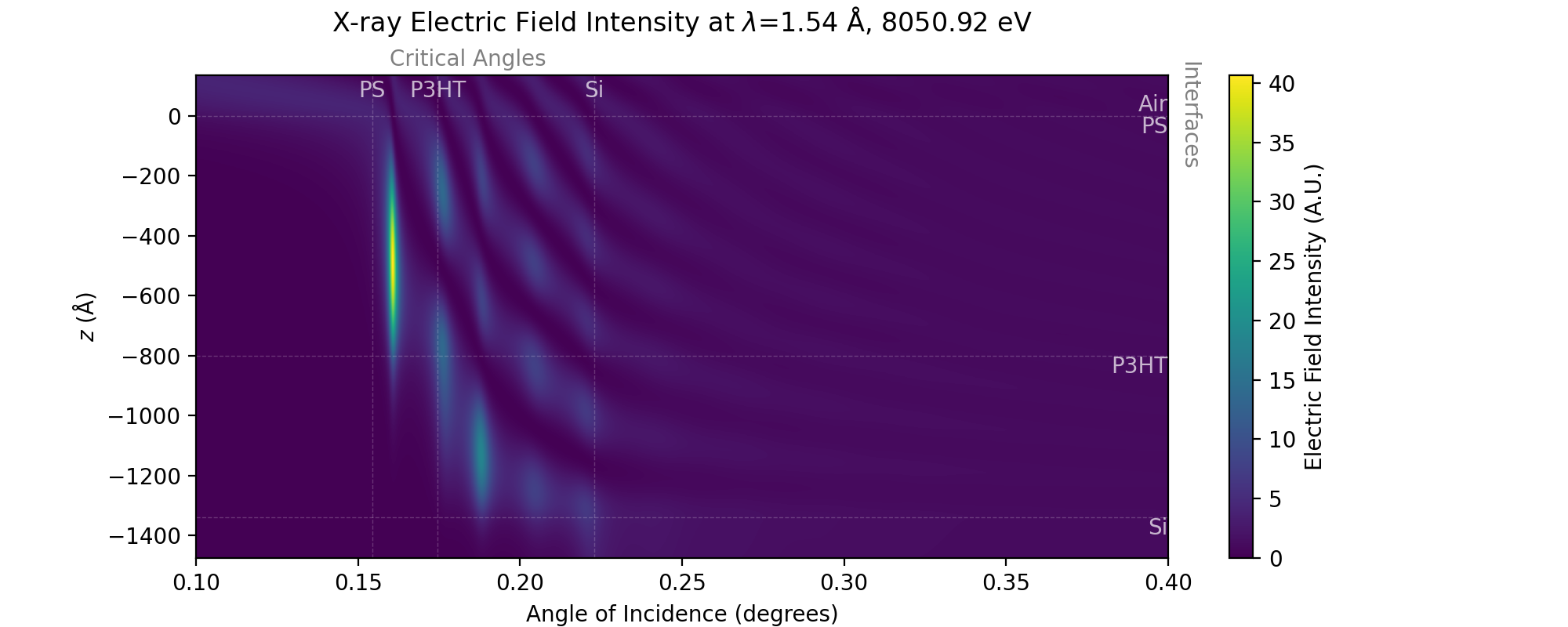
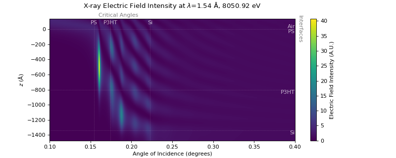
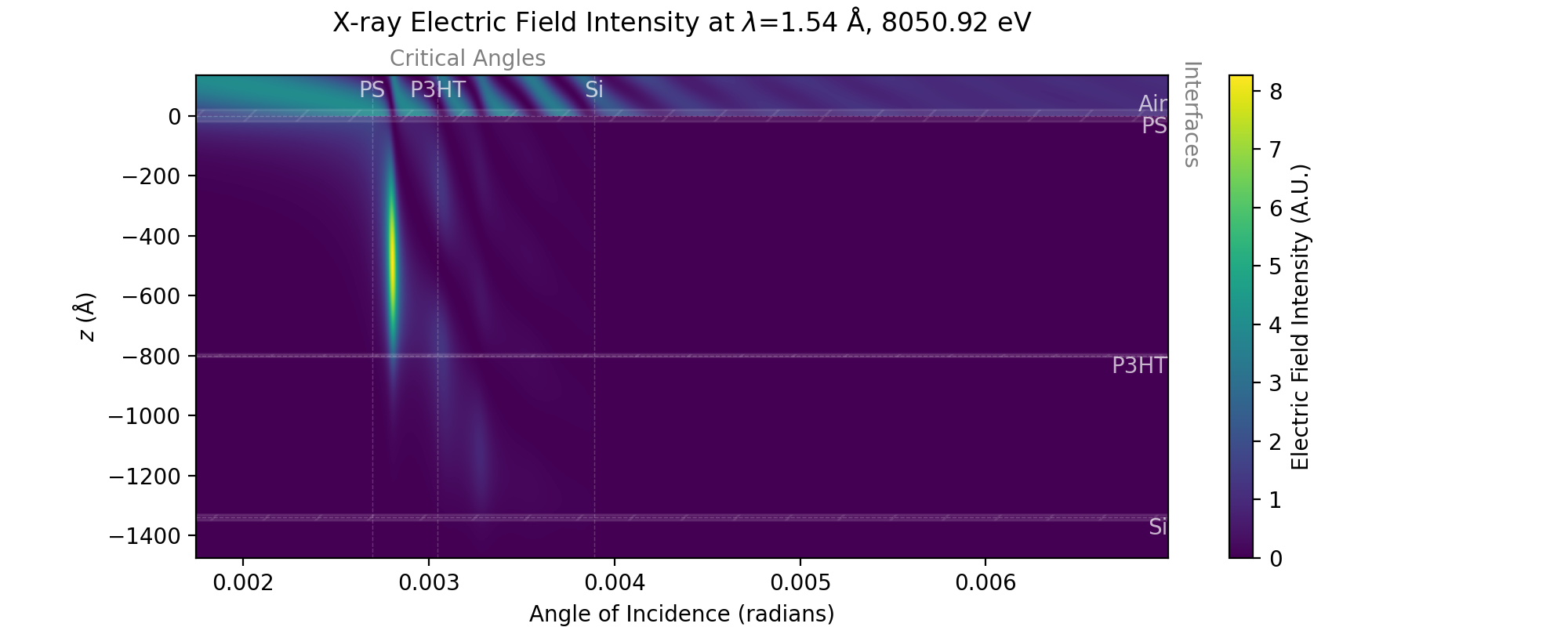
This includes the electric field intensities, both reflected and transmitted, at each interface, which allows us to calculate the total electric field intensity at any depth within the multi-layer structure, and subsequently can be used to generate the XEFI maps or depth dependent intensity summations.
# Can provide z_vals argument to specify depth values for the map,
# but by default plots extra 10% of the total thickness into the semi-infinite layers.
fig, ax = result.generate_graphic_XEFI_map()
ax.set_title(
    rf"X-ray Electric Field Intensity at $\lambda$={XEFI.utils.en2wav(energy):0.2f} Å, {energy:0.2f} eV",
    pad=20,
)
plt.show()
(Source code, png, hires.png, pdf)
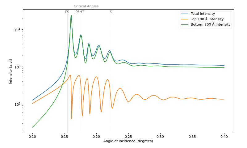
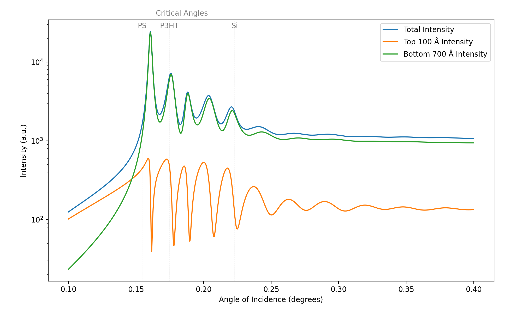
Intensity Summation#
The XEFI map can be integrated over depth to calculate the total intensity within each layer, which is useful for calculating the expected fluorescence or photoelectron yield from each layer.
intensity_full = result.summed_intensity(np.linspace(0, -800, 1000))
top_depth = 100
intensity_top = result.summed_intensity(
    np.linspace(0, -800, 1000), bounds=(0, -top_depth)
)
intensity_bot = result.summed_intensity(
    np.linspace(0, -800, 1000), bounds=(-top_depth, -800)
)

fig,ax = plt.subplots()
ax.plot(angles, intensity_full, label="Total Intensity")
ax.plot(angles, intensity_top, label=f"Top {top_depth} Å Intensity")
ax.plot(angles, intensity_bot, label=f"Bottom {800 - top_depth} Å Intensity")
ax.set_xlabel("Angle of Incidence (degrees)")
ax.set_ylabel("Intensity (a.u.)")
ax.set_yscale("log")
ax.legend()
plt.show()
(Source code, png, hires.png, pdf)

BasicRoughResult#
We can also add roughness rather simply by modifying the XEF_Basic call to generate a BasicRoughResult object. In the background, supplying interface roughness values modifies the Fresnel coefficients, which perturbs the recursive algorithm.
.. with the Nevot-Croce factor.
Here we arbitrarily choose roughness values of 20 Å, 5 Å, and 10 Å for the three interfaces respectively (Air/PS, PS/P3HT, P3HT/Si).
result_rough: XEFI.BasicRoughResult = XEFI.XEF_Basic(
    energies=energy,
    angles=angles,
    z=z,
    refractive_indices=refractive_indices,
    layer_names=layer_names,
    z_roughness=[40, 10, 20], # Roughness values for each interface in Å
)
This will generate a new result object with the roughness included in the calculation, which can be plotted in the same way as the smooth result. Note that we can turn on / off the grid for roughness values in the map using the grid_roughness argument in the plotting method.
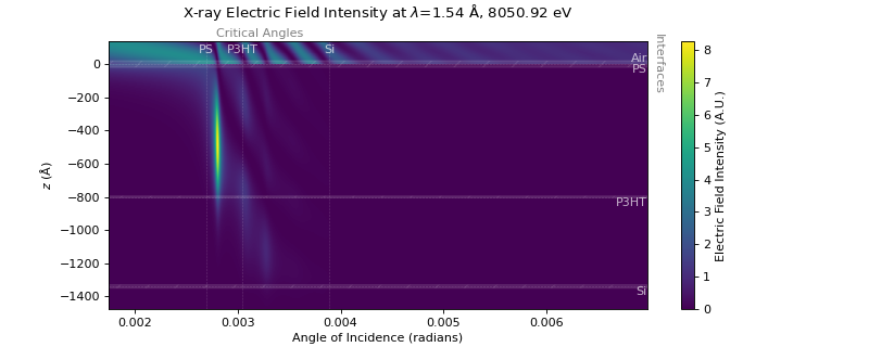
fig, ax = result_rough.generate_graphic_XEFI_map(
    grid_roughness=True,
    angles_in_deg=False,
)
ax.set_title(
    rf"X-ray Electric Field Intensity with Roughness at $\lambda$={XEFI.utils.en2wav(energy):0.2f} Å, {energy:0.2f} eV",
    pad=20,
)
plt.show()
(Source code, png, hires.png, pdf)
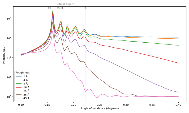
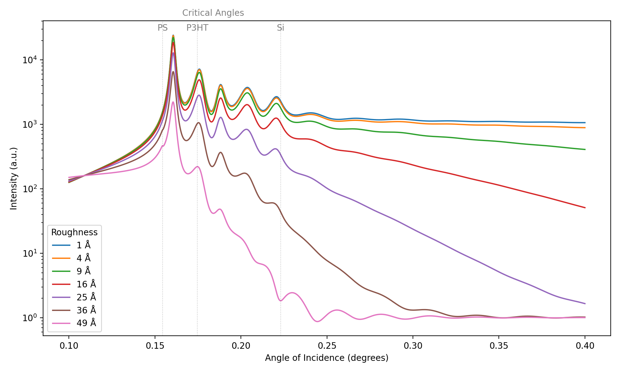
We can then calculate the changing intensity within a rough film (say Polystyrene) by modifying the interface roughness and repeating the summation.
fig, ax = plt.subplots(figsize=(10,6))
for roughness in [1, 4, 9, 16, 25, 36, 49]:
    result_rough: XEFI.BasicRoughResult = XEFI.XEF_Basic(
        energies=energy,
        angles=angles,
        z=z,
        refractive_indices=refractive_indices,
        layer_names=layer_names,
        z_roughness=[roughness, roughness, roughness], # Roughness values for each interface in Å
    )
    intensity_rough = result_rough.summed_intensity(np.linspace(0, -800, 1000))
    ax.plot(angles, intensity_rough, label=f"{roughness} Å")

result_rough._add_crit_angles(ax=ax)

ax.set_xlabel("Angle of Incidence (degrees)")
ax.set_ylabel("Intensity (a.u.)")
ax.set_yscale("log")
ax.legend(title="Roughness", loc="lower left")
plt.show()
(Source code, png, hires.png, pdf)
