Sliced#
The XEF_Sliced model allows for the calculation of the electric field intensity within a film by slicing it into many thin layers and summing the contributions from each layer. This is particularly useful for understanding how the intensity changes within a film, especially when there are rough interfaces, an alternative method to the XEF_Basic model with roughness (Basic Roughness Model).
Because the film is sliced into many layers, the specified z-coordinates do not match the actual z-coordinates of the layers used in the calculation. This changes the model parameters, to include new attributes:
pre_z: The original z-coordinates supplied by the user, which are used to define the geometry of the model.z: The z-coordinates of the sliced layers, which are used in the calculation of the electric field intensity.pre_N: The number of layers defined by the user, which is one less than the length of thepre_zlist.N: The number of sliced layers, which is determined by the slice_thickness parameter and the total thickness of the film.slice_thickness: The thickness of each slice, which determines how many layers the film is sliced into.sigmas: The number of standard deviations to include in smoothing between layers. This extends the z-range of the model to include the tails of the Gaussian smoothing function, which can be important for accurately modeling rough interfaces.
Let’s define some initial parameters, like in the basic model. We can define the geometry and refractive indices of the layers. However, we also need to specify how the refractive index changes through the sliced distribution.
import XEFI
import numpy as np

energy = 8050.92 # eV, corresponding to a wavelength of 1.54 Å
angles = np.linspace(0.1, 0.4, 3000) # Angles of Incidence in degrees
z = [0, -800, -1340]  # Z-coordinates for the multilayer interface
layer_names = ["Air", "PS", "P3HT", "Si"]
We can now define the refractive indices for each layer. See KKCalc2 for how to calculate these using the kkcalc2 package.
# Calculated at 8050.92 eV using kkcalc2, but could be any complex
# refractive index or callable that returns a complex refractive index.
refractive_indices = [
    1.0        + 0j,         # Air/Vacuum
    0.99999637 + 4.96e-09j,  # Polystyrene (C8H8)
    0.99999536 + 3.31e-08j,  # Poly(3-hexylthiophene) (P3HT, C10H14S)
    0.99999243 + 1.72e-07j,  # Silicon (Si)
 ]
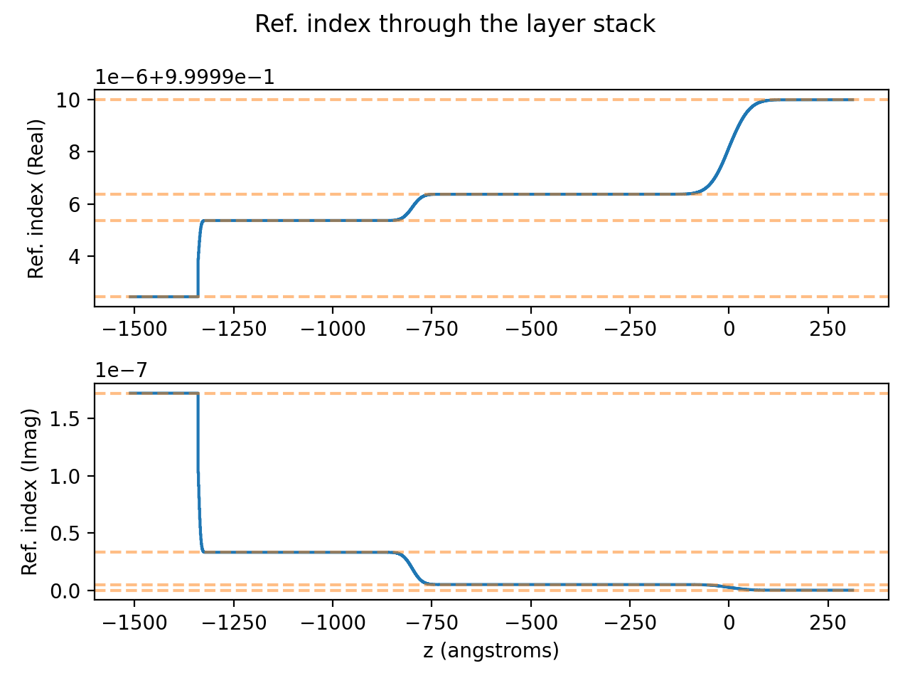
Functionalizing the interface#
To use the XEF_Sliced model, we again supply roughness values for each film interface. In the background, the model will slice the film into many thin layers, and apply a Gaussian smoothing function to the refractive index distribution to create a smooth transition between layers. The width of this smoothing function is determined by the roughness values supplied, and the number of slices is determined by the slice_thickness parameter.
result = XEFI.XEF_Sliced(
energies=energy,
angles=angles,
z=z,
refractive_indices=refractive_indices,
z_roughness=[40, 20, 5],
slice_thickness=1.0,
sigmas=4.0,
layer_names=labels,
)
ax = result.graph_refractive_indexes()
ax[0].figure.tight_layout()
plt.show()
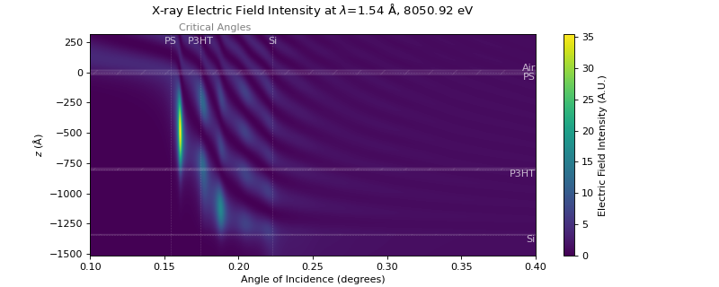
# Can provide z_vals argument to specify depth values for the map,
# but by default plots extra 10% of the total thickness into the semi-infinite layers.
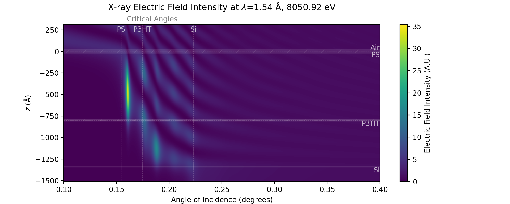
fig, ax = result.generate_graphic_XEFI_map()
ax.set_title(
rf"X-ray Electric Field Intensity at $\lambda$={XEFI.utils.en2wav(energy):0.2f} Å, {energy:0.2f} eV",
pad=20,
)
plt.show()
(Source code, png, hires.png, pdf)

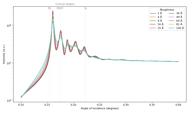
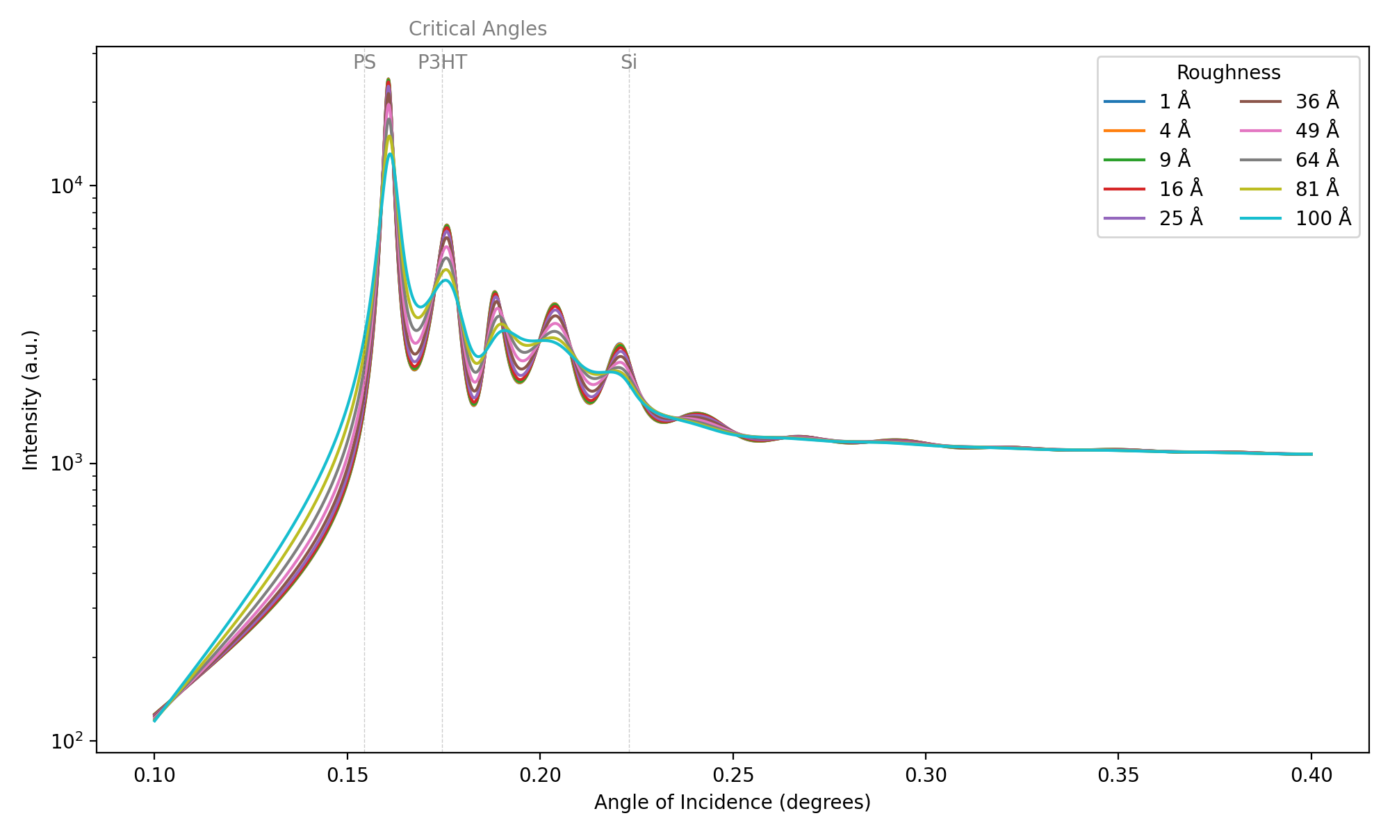
Thickness Variation#
The sliced model inherently calculates changes with thickness differently to that of the basic model.
fig, ax = plt.subplots(figsize=(10,6))
for roughness in [1, 4, 9, 16, 25, 36, 49, 64, 81, 100]:
    result_rough: XEFI.SlicedResult = XEFI.XEF_Sliced(
        energies=energy,
        angles=angles,
        z=z,
        refractive_indices=refractive_indices,
        z_roughness=[roughness, roughness, roughness],
        slice_thickness=1.0,
        sigmas=4.0,
        layer_names=layer_names,
    )
    intensity_rough = result_rough.summed_intensity(np.linspace(0, -800, 1000))
    ax.plot(angles, intensity_rough, label=f"{roughness} Å")

result_rough._add_crit_angles(ax=ax)

ax.set_xlabel("Angle of Incidence (degrees)")
ax.set_ylabel("Intensity (a.u.)")
ax.set_yscale("log")
ax.legend(title="Roughness", loc="upper right", ncol=2)
plt.show()
(Source code, png, hires.png, pdf)